The textbook does cover MIP, but there are many free (and non-free)
resources. To do the assignment reader the slides is probably enough,
but the following links are helpful.
Again the book does not cover Stochastic local search. The slides
should contain enough material to complete the assignment. but you
can look at Coursera course Solving Algorithms for Discrete
Optimisation. The
book Stochastic Local
Search
is a good general reference.
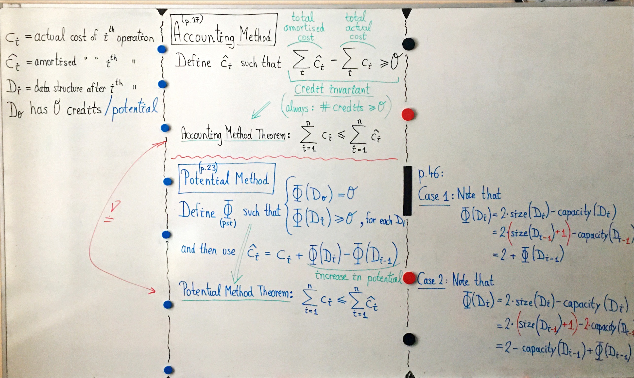
Amortised analysis can be quite difficult to understand first time
around. The slides contain a lot of material and examples, but you are
also encouraged to read Chapter 16 of the textbook. There are a few
takeaways from this lecture
Amortised analysis is the time needed (in the computational
complexity $O()$ sense) to do any sequence of $n$ operations, and
hence gives you the average time complexity of a single operation.
You can brute force the mathematics and just compute the complexity
or can use the Accounting Method or the Potential method.
Both the accounting method and the potential method give you
mathematical tricks to estimate the total computational complexity for
a sequence of $n$ operations.
In the lecture we will look at
A rather artificial example of a stack where you can remove $k$
items in one go.
A binary counter
A more useful dynamic table, that can resize itself as it gets full.
The binary counter and the stack are useful to understand how the
accounting or potential method work. The dynamic table is the
foundation of many modern data-structures.
Today we are going to look at probabilistic analysis of
algorithms and some techniques for designing algorithms that use
randomisation. Randomised algorithms is a big subject, which has many
useful and efficient algorithms. Unfortunately, we will only scratch
the surface.
We will cover
The hiring problem as a prototypical probabilistic problem
Indicator Variables
Linearity of expectation. Given two random variables $X$ and $Y$,
then the expectation $E(X + Y) = E(X) + E(Y)$. The theorem is true
for any distribution of $X$ and $Y$. This is perhaps one of the most
useful theorems in probabilistic analysis of algorithms.
Some examples of using indicator variables including the hat
problem, the birthday paradox.
Some randomised strategies for the hiring problem, or using
randomness to avoid worst case run times.
The algorithm for generating random permutations uniformly. We will
not cover the proof of its correctness.
Analysis of Hash tables including expected load factors and chain
length.
Universal Hashing. A randomised technique to build efficient hashing
functions.
Slides
The information in the slides is spread out all over the place. I plan
to use the whiteboard. You are better off looking at the textbook, but
take a look at
The slides contain a lot of material. You are strongly advised to read
the textbook.
Chapter 5 contains the relevant background on probabilistic
analysis and randomised algorithms
Chapter 11 up to and including 11.3.4 has the material on hash
tables. Some of this material should be revision.
Appendix C contains some background on probability that you might
need to refer to while reading the other material.
Lecture 6
Today we are going to look at polynomial time reductions between
problems. We will use some of the slides from
here. Exactly
what we cover depends on how much time we have and what the interest
of the class is. You are advised to read all of the slides and the
corresponding material in the book. Chapter 34 is essential reading
for both today’s lecture and Lecture 9.
There are two motivations for studying polynomial time reductions:
If I have an algorithm for one problem, then I can use it to solve
other problems that on the surface seem different.
To study the computational complexity of polynomial and
non-deterministic problems. If I know that my problem is NP-hard, then
I am very unlikely to find a polynomial time algorithm.
Today we will be thinking more about the first case, and in Lecture 9
we will look more at the landscape of computational complexity.
Reading Material
All of Chapter 34
Lecture 7
Slides and Topics
Today is a flipped lecture on SAT. This lecture will
prepare you for problem 3 of assignment 2.
Watch the following videos. The cover slides 1-29 of
SAT-intro
and slides 1-4 of
SAT-CDCL.
Today we will look at approximation algorithms. This is another way of
dealing with NP-completeness. We find a polynomial time algorithm
(often greedy) that is guaranteed to find an solution within some
bound or ratio of the optimal solution.
Lecture plan
I am not sure how many of the slides I will use. Some of the material
is easier on the whiteboard. The slides are only a guide. To master
the material you should read the book.
After covering the definitions we will look at a number of techniques
for developing approximation algorithms:
Greedy algorithms: node/vertex cover and set-covering. Often by
analysing the naive greedy algorithm you can work out the
approximation ratio.
Using existing algorithms to compute something that can be
transformed into a solution. Using Minimum Spanning Trees to
solve certain classes of TSPs.
Proving that there are no approximation algorithms for certain
NP-complete problems.
Derandomisation: Use a randomised algorithm, but remove the
randomness to get a polynomial time algorithm. We look at
approximation algorithms for Max-SAT.
TBA, more approximation algorithms. I would like to cover
set-covering, but some of the maths gets a bit involved, and you
need to take some calculus/analysis on trust.
These
Slides
from CMU cover the metric travelling salesperson problem.
Slides
from Cambridge, UK
that cover the proof that there is no approximation algorithm with
ratio greater than or equal to 1 for TSP unless P equals NP.
Assignments
Help, Solution, and Grading Sessions and Guide for the Perplexed.
The course has 2 mandatory assignments, to be done in teams of two. The
assignments are worth 2 higher-education credits (ECTS credits) in
total.
Help Sessions,
Each assignment has 3 timetabled help sessions. Help sessions are
the only time that you can help from the assistants. We will not
give support at other times.
Initial Grading
For each problem of an assignment, your initial score, in the
integer interval $0 \ldots 5$, will normally be determined by the late
afternoon on the day before the grading session for that
assignment. Toward this, the assistants run your code on a grading
test suite and examines the corresponding part of your report. An
initial score is the final score if it is greater than or equal to
$3$.
Grading Session
The objective of a grading session is to determine your final score
for each problem with an initial of 1 or 2: your team will
normally be given an appointment with an assistant during the grading
session, in a room of her/his choice, toward correcting minor
mistakes during that meeting and possibly increasing your score by one
Appointment times are strict: the initial score is final in case
of a missed appointment. Exceptions must be negotiated in due time
during working hours with the head teacher, upon reporting a convincing
case of force majeure.
Solution Sessions
The objective of a solution session is only for the assistants
to discuss acceptable solutions to the assignment of the previous
deadline. No code will be handed out. The first solution
session is merged with the initial help session to the second
assignment.
Comments on your submitted report can be found at Studium; more detailed
comments can be obtained orally from the assistants upon appointment.
Submission and Deadlines
All assignment reports must be submitted via Studium. Submission
deadlines are hard. The submission deadline and time in Studium
is always correct (if it differs from information on this webpage).
Exceptions must be negotiated in due time during working hours with
the head teacher, upon reporting a convincing case of force
majeure. Grading will only start after a deadline, so you can submit
multiple times until then.
Ethics
The legislation on plagiarism and
cheating
(summary) of Uppsala
University will be rigorously applied, without exceptions. This
disallows using a public repository (such as GitHub, where you should
use a free private student
repository) for code management
within your team. We reserve the right to use plagiarism detection
tools and point out that they are extremely powerful.
Your report should be your own work, and not the product of a large
language model. You should do the assignments without the use of an AI
coding assistant.
When submitting you implicitly certify that your report and all its
uploaded attachments were produced solely by your team, except where
explicitly stated otherwise and clearly referenced, that each teammate
can individually explain any part starting from the moment of
submitting your report, and that your report and attachments are not
freely accessible on a public repository.
We reserve the right to give different assignment scores to the
teammates of a team, depending on the performance at the grading
session.
Please report any problems within a team to the head teacher, who will
handle the case in confidence, in the best interest of both teammates,
keeping the ethics dimension in mind.
Expected Effort
One higher-education credit (ECTS credit) translates under Swedish
university law into an expected 26.67 hours of work for the average
student. Hence 133.33 hours are expected on this 5-credit course.
The assignments are worth 2 credits in total. Not counting the 21 hours
spent on attending the lectures, the 2 assignments are calibrated to
take an average of 30 hours each, for the average student, for each
teammate, including the corresponding help, grading, and solution
sessions.
Do not expect the 2 assignments to be equally labour-intensive, and do
not expect the 2 problems of each assignment to be equally
labour-intensive.
Effortless and free access to MIP solvers is provided by the NEOS
Server for Optimisation
(search for “mixed integer linear programming”). We then recommend
you use the world-class commercial MIP solver Gurobi
Optimizer (or, but only in case of a
temporary licensing issue with Gurobi at NEOS, the open-source MIP
solver HiGHS), via the AMPL
modelling language: when using the NEOS server, you do not need to
install the AMPL integrated development environment (IDE) or AMPL
command-line interface (CLI) or a MIP solver. Use a commands file
with option gurobi_options 'outlev=1'; solve; # Write display commands here: display ___; in order to turn on verbose
printing, which includes the optimality gap.
The effort of installing the following free alternative is outside
the course time budget (and we have no resources to help you with
installation issues), since NEOS provides access to installed
versions:
If you have and prefer to use your own hardware, then you can
install AMPL bundled with Gurobi Optimizer
by following by using the courses classroom licence. When this is
available there will be instructions in the file
installing-AMPL.txt in the Files section at the AD3 page of
Studium: a course license was provided free-of-charge by
AMPL.com. Use AMPL command option solver gurobi; option gurobi_options 'outlev=1'; before you run solve in
order to turn on verbose printing, which includes the optimality
gap.
If the class licence is not available, then you can download a free
time limited version from AMPL.com. Using your
academic email address it is possible to get an academic licence.
The AMPL book can be downloaded
free of charge, but you normally do not need to read it, as the
sample models on the lecture slides suffice.
We recommend you use the SAT solver MiniSat. Use
the DIMACS
CNF
format for SAT solvers, by DIMACS, the
Center for Discrete Mathematics and Theoretical Computer Science.
There is a 5-hour long individual, written, closed-book exam at
the end of the course, where you can only use blank paper, pencils, and
an eraser, that is no help: no books, no slides,
no notes, no electronic devices, etc:
Exam: at the end of period 3, please see Ladok, and don’t forget
to register for the exam.
First re-exam: June 2025, time and place to be announced
Second re-exam: August 2025, time and place to be announced
There will be a question on establishing NP-completeness for some
problem, and at least half the points of that question must be earned in
order to pass the exam. The exam questions will be drawn from the
following list or will be very similar to questions in this list:
Probabilistic Analysis: Exercises 5.2-{1,2,5,6} of CLRS4.
Randomised Algorithms: Exercises 5.3-{2,3,4} of CLRS4.
Amortised Analysis: Exercises 16.1-{1,3} of CLRS4; Exercises
16.2-{1,2} of CLRS4; and Exercise 16.3-2 of CLRS4.
NP-Completeness: Exercise 34.5-2 of CLRS4 by following the hint
in one step; Exercises 34.5-{5,6,7} of CLRS4; Problem 34-1ab of
CLRS4 by following the hint in one step; Exercise 35.3-2 of CLRS4;
and Problem 35-1a of CLRS4 by following the hint in one step;
exercises not in CLRS4 (version of
2025-06-19).
Approximation Algorithms: Exercises 35.1-5 of CLRS4; Exercise
35.4-2 of CLRS4; and Problems 35-{1bcde,3} of CLRS4.
Since it is a closed-book exam, the questions will be asked in a
self-contained way.
Exam study groups are allowed and even encouraged, as the exam is
individual. The exam topics are taught as early as possible towards
maximising the time available for exam preparation. Exam preparation
sessions under the supervision of the head teacher (and assistants)
cannot be organised, as that would 'burn' the CLRS4 questions tackled
in such sessions.
Expected Effort
One higher-education credit (ECTS credit) translates under Swedish
university law into an expected 26.67 hours of work for the average
student. Hence 133.33 hours are expected on this 5-credit course.
The exam is worth 3 credits. The actual preparation and taking of the
exam are expected to take 52 hours. Recall also that 21 hours are spent
on attending the lectures and that 60 hours are expected on working for
the 2 credits for the
assignments.
All this does not clash with other courses you are taking, as university
studies are legally defined to take 400 hours of work per study period
(normally 10 weeks), and the standard 15 credits targeted in a study
period are calibrated to reach that total.
Grades and Credits
Grades and Credits
The two assignments are worth 2 higher-education credits (ECTS credits).
The assignment grade is as follows where $a_i$ is the final score
of assignment $i$.
Grade
Condition
5
$18 \leq a_1 + a_2 \leq 20$, no problem score $0$, guest lecture attened and $a_1,a_2 \geq 3$.
4
$14 \leq a_1 + a_2 \leq 17$, no problem score $0$, guest lecture attened and $a_1,a_2 \geq 3$.
3
$10 \leq a_1 + a_2 \leq 13$, no problem score $0$, guest lecture attened and $a_1,a_2 \geq 3$.
A missed guest lecture (in case of no force majeure) can be
compensated for by a summary of a research paper chosen by the head
teacher.
The exam is worth 3 higher-education credits (ECTS credits). The exam
grade is as follows when $e$ is your exam score (out of 20):
Grade
Condition
5
$18 \leq e \leq 20$
4
$14 \leq e \leq 17$
3
$10 \leq e \leq 13$
U
$0 \leq e \leq 9$
The overall grade is as follows when you have earned the 2
assignment credits with total score
Grade
Condition
5
$86 \leq 2a + 3e \leq 100 \land a \geq 10 \land e \geq 10$
4
$66 \leq 2a + 3e \leq 85 \land a \geq 10 \land e \geq 10$
3
$50 \leq 2a + 3e \leq 65 \land a \geq 10 \land e \geq 10$
If the resulting grade is lower than your exam grade, then the overall
grade is the exam grade.
These rules are effective as of Mon 19 Jan 2026. The head teacher
reserves the right to modify them at any moment, should special
circumstances call for this.
We highly recommend you learn or use LaTeX for typesetting your
assignment reports and presentation slides in a professional way, but
this is optional. The learning of LaTeX is outside your time
budget for this course, but very well-invested as you will find out
during the course or later. Here are some LaTeX resources:
Our provided skeleton reports also contain examples of all LaTeX
commands you need for this course; from the command line (or with
Emacs/Aquamacs), compile with pdflatex (once or twice, depending
on whether cross-references need to be recomputed), and run bibtex
whenever the bibliography was modified