Lecture 4

Today we are going to look at amortised analysis.

• slides
• demo of the dynamic table

Amortised analysis can be quite difficult to understand first time around. The slides contain a lot of material and examples, but you are also encouraged to read Chapter 16 of the textbook. There are a few takeaways from this lecture

• Amortised analysis is the time needed (in the computational complexity $O()$ sense) to do any sequence of $n$ operations, and hence gives you the average time complexity of a single operation.
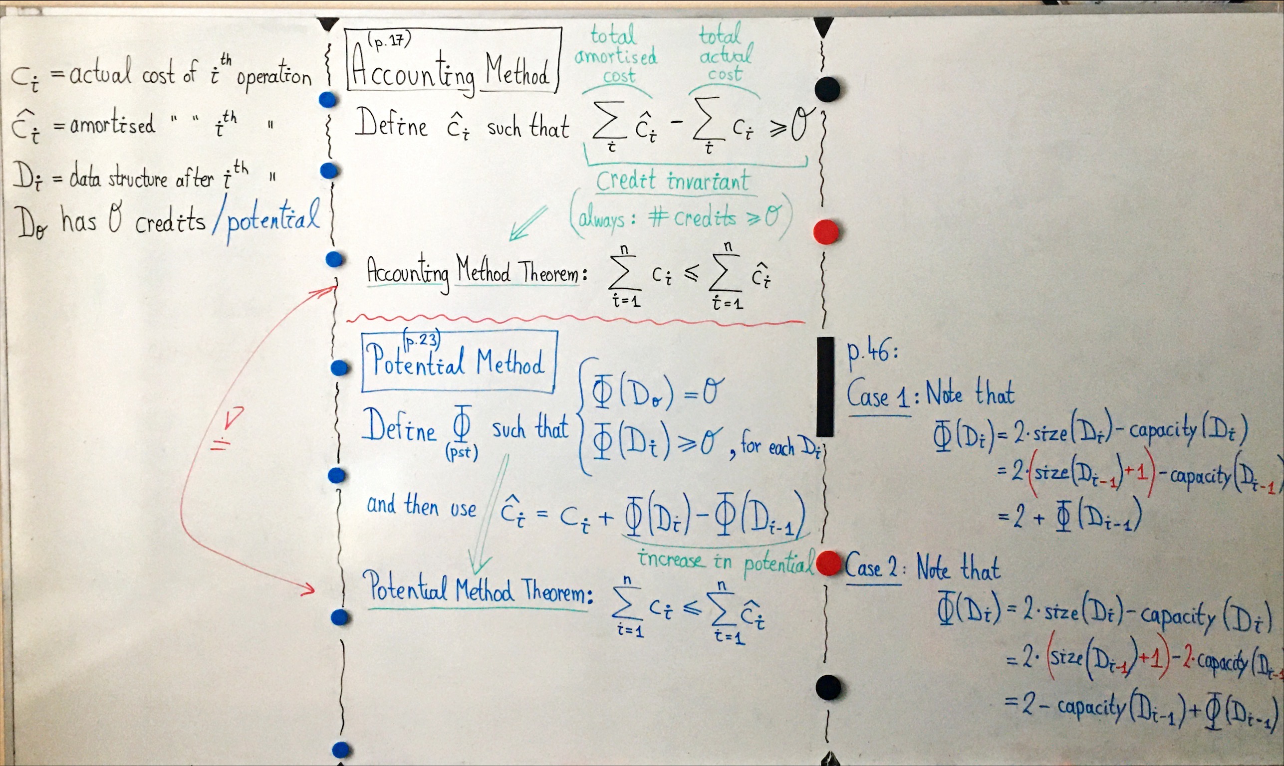
• You can brute force the mathematics and just compute the complexity or can use the Accounting Method or the Potential method.

Both the accounting method and the potential method give you mathematical tricks to estimate the total computational complexity for a sequence of $n$ operations.

In the lecture we will look at

• A rather artificial example of a stack where you can remove $k$ items in one go.
• A binary counter
• A more useful dynamic table, that can resize itself as it gets full.

The binary counter and the stack are useful to understand how the accounting or potential method work. The dynamic table is the foundation of many modern data-structures.

You might find Pierre Flener’s whiteboard notes useful.